How to measure your supply chain performance variability

In a previous article, we explained why probabilistic planning is important and how it adds value to your decision-making. By nature, stochastic insights are complicated to understand, especially for practitioners who are not necessarily familiar with the typical statistical measures of variability. Transparent metrics that clearly communicate the impact of variability are essential to helping decision makers understand how variation on the input side influences variation on the performance side. Even more important is for them to understand how tactical decisions affect that uncertainty profile. In this article, I go a bit deeper into how supply chain performance variability can be measured.

Traditional measures of variability

It is, of course, not news that variability has a tremendous impact on supply chain performance. By the 1980s and ‘90s, the negative consequences of supply chain performance variability were already a key driver behind Total Quality Management and 6σ (Six Sigma) movements, with new statistical methods being popularized in an attempt to better quantify that variability (and therefore help to mitigate its effects).

When statisticians measure variability, very often you encounter one of the following metrics:

• Range: The range is the difference between the largest and smallest values in a dataset. It is easy to calculate and understand but it is sensitive to outliers and does not take into account the distribution of values within the dataset.
• Interquartile range (IQR): The IQR is the difference between the third quartile and the first quartile of a dataset. It is more resistant to outliers than the range but it is still sensitive to the presence of extreme values.
• Variance: The variance is a measure of how spread-out the values in a dataset are. It is calculated by taking the sum of the squares of the differences between each value and the mean of the dataset, and then dividing by the number of values in the dataset. The variance is useful for comparing the spread of different datasets but it can be difficult to interpret because it is in units that are squared.
• Standard deviation: The standard deviation is the square root of the variance, and it is a measure of how spread out the values in a dataset are. It is easier to interpret than the variance because it is in the same units as the original data. However, it is still sensitive to outliers and can be affected by the presence of extreme values.
• Coefficient of variation: The coefficient of variation is the standard deviation divided by the mean of a dataset. It is a measure of the relative spread of a dataset and is useful for comparing the spread of datasets with different units or means. However, it does not take into account the shape of the distribution and can be affected by the presence of extreme values.
• Confidence intervals: Confidence intervals are a way to estimate the range in which a population parameter is likely to fall. They are typically constructed by calculating a sample statistic (such as the mean or median) and then adding and subtracting a margin of error based on the standard error of the statistic and the desired level of confidence. Confidence intervals can be used to quantify the uncertainty associated with an estimate and to compare the precision of estimates from different samples.

→ While these are very useful measures to describe the inputs to your supply chain environment, they may not necessarily be sufficient to describe the performance of your supply chain.

Going one step deeper

While these traditional metrics offer some insight into statistical behaviors, supply chain performance is the result of complex interactions between many sources of variability/uncertainty and so basic methods can only ever provide guidance, rather than genuine insights into real world events. That’s why more advanced methodologies must be employed to deliver greater value, including:

• Bootstrapping: This is a resampling technique that can be used to estimate the sampling distribution of a statistic. It involves repeatedly drawing random samples with replacement from a dataset and calculating a statistic of interest for each sample. The resulting distribution of statistics can be used to construct confidence intervals, to perform hypothesis tests or as an input for Monte Carlo simulations.
• Monte Carlo simulation: This is a computational technique that involves generating random samples from one or more probability distributions in order to estimate some quantity of interest. They can be used to explore the uncertainty associated with different assumptions or models and to compare the outcomes of different scenarios.

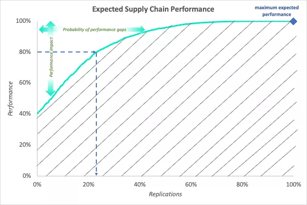
Monte Carlo simulations are instrumental in creating expected performance graphs and their related “area under the curve” (AUC) metric. While AUC has its origin in the machine learning community, the idea has been adapted to give a clear insight in the probabilistic behavior of supply chain performance.

The traditional AUC curve is one of the most important evaluation metrics for checking any classification model’s performance. It maps the false positive rate on the X-axis versus the true positive rate on the Y-axis, and the AUC is then calculated by finding the area under this curve. This is done by approximating the curve using a series of straight line segments and summing the area of the resulting trapezoids. The higher the AUC, the better the performance of the classifier.

When measuring supply chain performance, we use AUC in a somewhat different way. By normalizing the number of replications of a Monte Carlo simulation on the one hand and creating normalized performance indicators on the other hand, we get a 100% by 100% framework that allows us to map performance per replication in an increasing way, as illustrated in the graph below:

This curve provides insight into the risk profile of the supply chain, and its key characteristics are as follows:

• The area under this curve gives insight into the expected performance under uncertain conditions;
• The intersection with the Y-axis indicates the minimum expected performance from the supply chain under the given input uncertainty. In other words, it tells you what impact you may experience in the worst case scenario. By drawing imaginary lines parallel to the Y-axis, you can derive additional insights about the performance percentiles;
• In the same vein, the Y-value of the curve where it intersects 100% on the X-axis tells you what the maximum achievable performance is;
• Interpreting the horizontal progression of the graph tells you something about the likelihood that things will happen:
  • The point on the X-axis for any performance level on the curve tells you how likely it is that performance will be lower than that point;
  • Conversely, by subtracting this value from 100%, you will see how likely it is that performance will be at least that high;
  • For instance, indicated by the blue arrows on the above graph, there is a 25% probability that performance will be below 80% (and thus a 75% probability that it will be at least 80%).

→ But how do we obtain this type of graph? Monte Carlo simulations are at the heart of the approach but how does that generate the expected range of future performance levels? More about that in a future article.